Clifford-Steerable Convolutional Neural Networks
Abstract
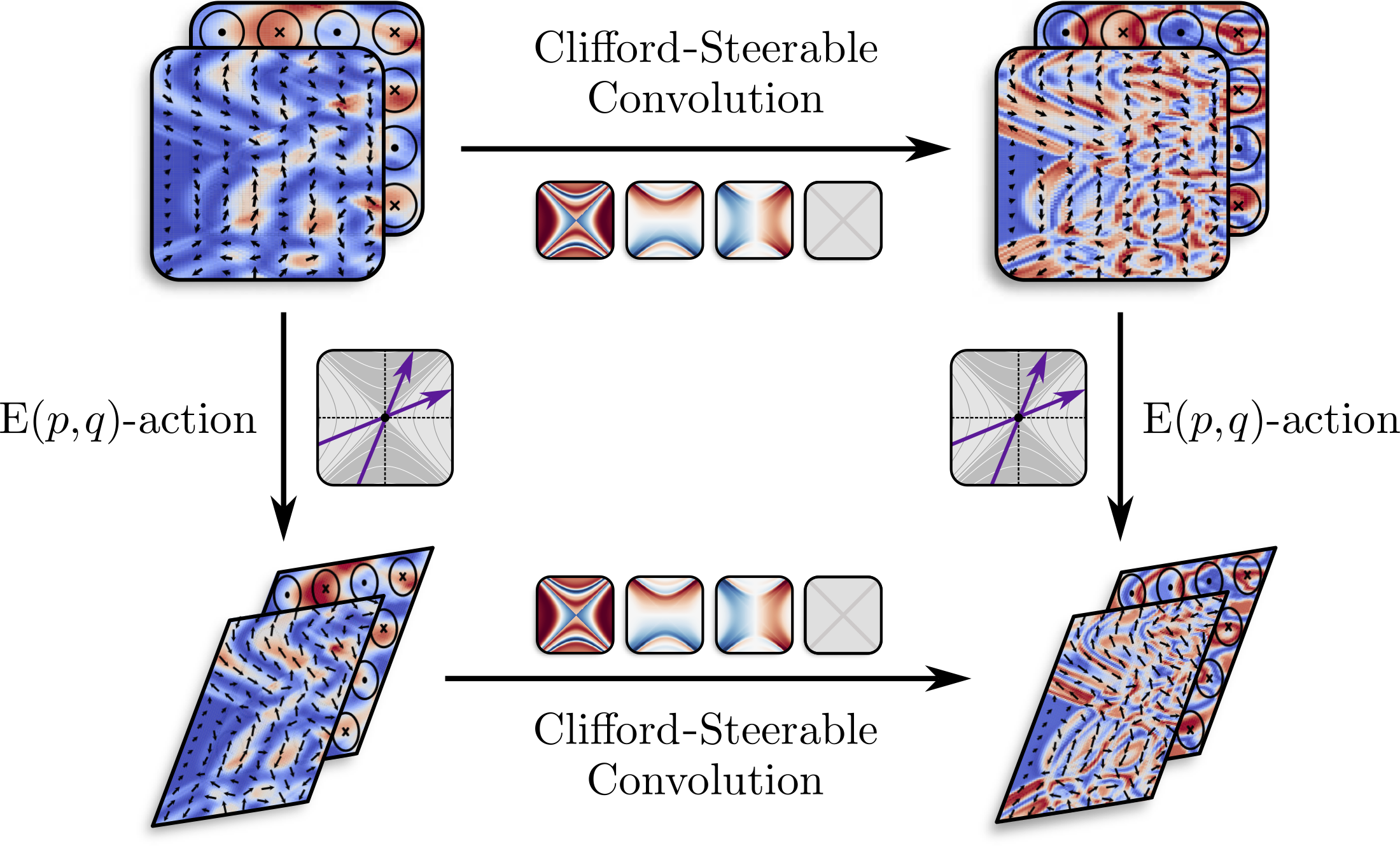
We present Clifford-Steerable Convolutional Neural Networks (CS-CNNs), a novel class of \(E(p, q)\)-equivariant CNNs. CS-CNNs process multivector fields on pseudo-Euclidean spaces. They cover, for instance, \(E(3)\)-equivariance and Poincaré-equivariance on Minkowski spacetime. Our approach is based on an implicit parametrization of \(O(p,q)\)-steerable kernels via Clifford group equivariant neural networks. We significantly and consistently outperform baseline methods on fluid dynamics as well as relativistic electrodynamics forecasting tasks.
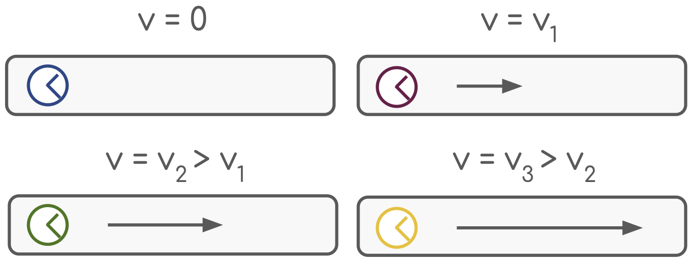
Clocks moving with different velocities in a rod.
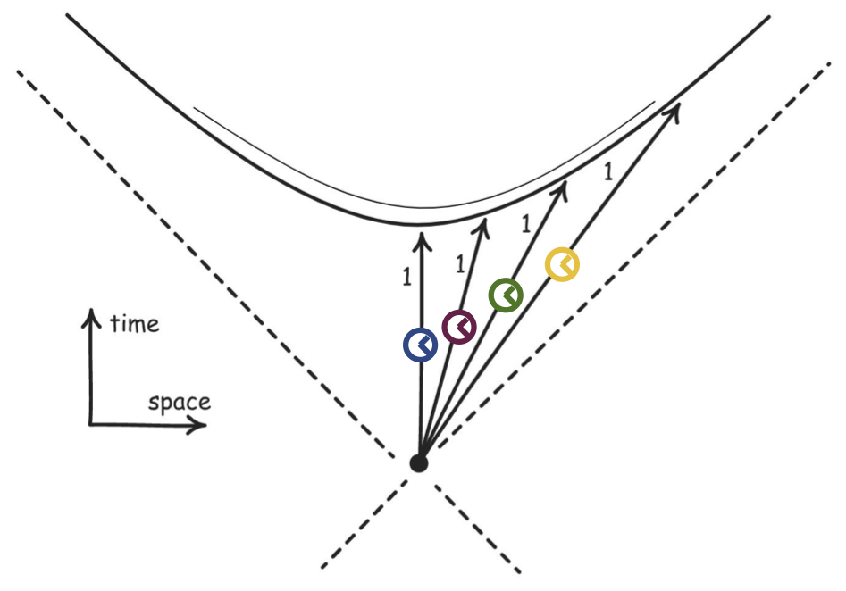
Spacetime diagram: where the clocks end up showing the same time.
Adapted from the blog post.
Spacetime
In classical physics, space and time are treated as separate entities: space is described using Euclidean geometry, and time is considered a continuous one-dimensional flow. This separation leads to different notions of distance in space and time. In space, to measure how far apart two points are from each other, we use the Euclidean distance: \[ d^2 = \Delta x^2 + \Delta y^2 + \Delta z^2 \] Time, on the other hand, is thought to be absolute: if we were to place two clocks at different locations, they would read the same time, regardless of their spatial separation or relative motion. In other words, the timing of events is assumed to be the same for all observers.
In relativistic physics, the situation is different. There, space and time are unified into a single entity - spacetime. It is described by Minkowski geometry, where the distance between two points is given by: \[ d^2 = c^2 \Delta t^2 - (\Delta x^2 + \Delta y^2 + \Delta z^2) \] where \(c\) is the speed of light. To better build an intuition, let us imagine four clocks moving at different velocities along a rod, and velocities are close to the speed of light. As time is compressed in the direction of motion at high velocities, the clocks have to travel longer distances to show the same time. If we now draw the trajectories of the clocks in spacetime, we would see that they end up on the same hyperbola. This hyperbola represents the set of all spacetime points that are separated from the origin by a fixed proper time interval.
Pseudo-Euclidean spaces
In the previous example, we saw that events at the same spacetime distance from an origin form a hyperbola in spacetime. This contrasts with Euclidean geometry, where points at the same distance from an origin form a circle in 2D or a sphere in 3D. In the right figure, you can visually compare the two geometries, with different colors representing loci of points at the same distance from the origin.
Minkowski spacetime differs from Euclidean space in that distances can be negative. Mathematically, it falls under the umbrella of pseudo-Euclidean spaces - a generalization of Euclidean spaces to include negative distances. Pseudo-Euclidean spaces are denoted as \(\mathbb{R}^{p,q}\), where \(p\) is the number of time-like dimensions and \(q\) is the number of space-like dimensions, and the tuple \((p,q)\) is called the signature of the space. Note that when \(p=0\) and \(q=3\), we obtain the 3D Euclidean space, and when \(p=1\) and \(q=3\), we obtain the 4D Minkowski spacetime.
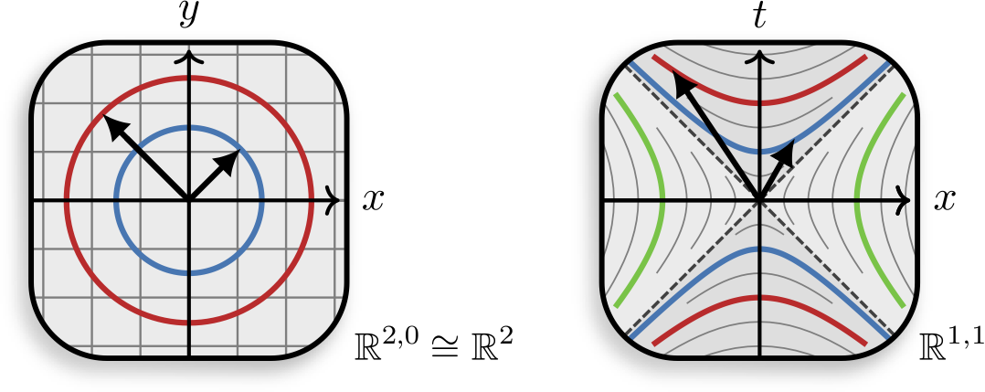
Euclidean space (left) and Minkowski spacetime (right). Colors depict different loci of points at the same distance from the origin.
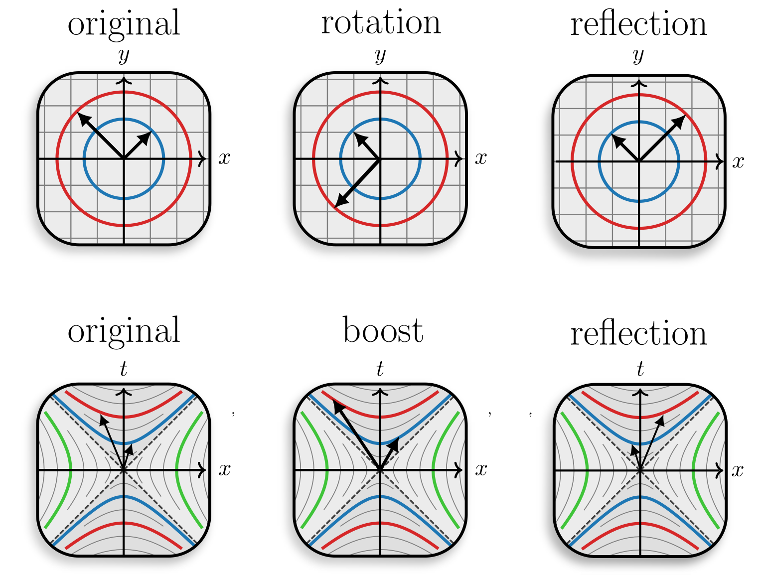
Isometry transformations of the Euclidean space (top) and Minkowski spacetime (bottom). Colors depict different loci of points at the same distance from the origin.
Isometries
We can now look at the transformations that preserve the distance in pseudo-Euclidean spaces - isometries. For Euclidean spaces, these are rotations, translations, and reflections which constitute the Euclidean group \(E(n)\). For pseudo-Euclidean spaces, the set of isometries includes translations, spatial rotations, reflections, and also boosts between inertial frames. They constitute the pseudo-Euclidean group \(E(p,q)\), which as special cases includes the Poincaré group for Minkowski spacetime \(E(1,3)\) and the Euclidean group \(E(0,n) \equiv E(n) \).
Mathematically, the pseudo-Euclidean group is defined as a semidirect product of the pseudo-orthogonal group \(O(p,q)\) (origin-preserving transformations) and the translation group \( (\mathbb{R}^{p+q}, +) \): \[ E(p,q) := O(p,q) \ltimes (\mathbb{R}^{p+q}, +). \] This means that any isometry can be represented as a composition of a linear transformation from the pseudo-orthogonal group \(O(p,q)\) and a translation.
Data on geometric spaces
We are interested in working with signals on spacetime, or any other geometric space. It is convenient to formalize data as functions from the space to some feature vector space \(W\): \[ f: \mathbb{R}^{p,q} \to W, \] to which we refer as feature vector fields. One can think of it as a function that assigns a feature vector to each point in the space, for example an RGB vector to each pixel in an image.
It is reasonable to assume that when a transformation \(g \in E(p,q)\) is applied to the input space \(\mathbb{R}^{p,q}\), it will also affect the feature vector field \(f\). To specify how the feature vector field \(f\) transforms under group actions \(g\), we equip it with a group representation \(\rho\): \[ [g.f](x) = \rho(g) f(g^{-1} x), \] where \(x \in \mathbb{R}^{p,q}\) is a point in the space. This equation essentially states that applying a transformation to the space and then evaluating the function is equivalent to evaluating the function first and then transforming its output. Common examples include scalar fields like grey-scale images and temperature distributions and vector fields such as wind velocity or electromagnetic fields.
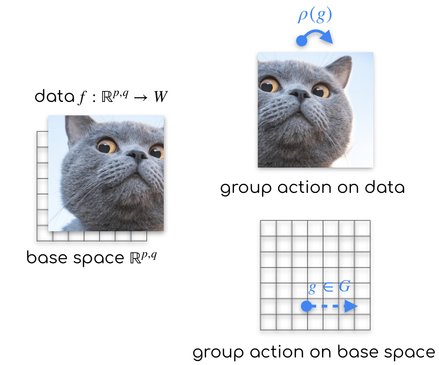
Group acts on data through group representations.
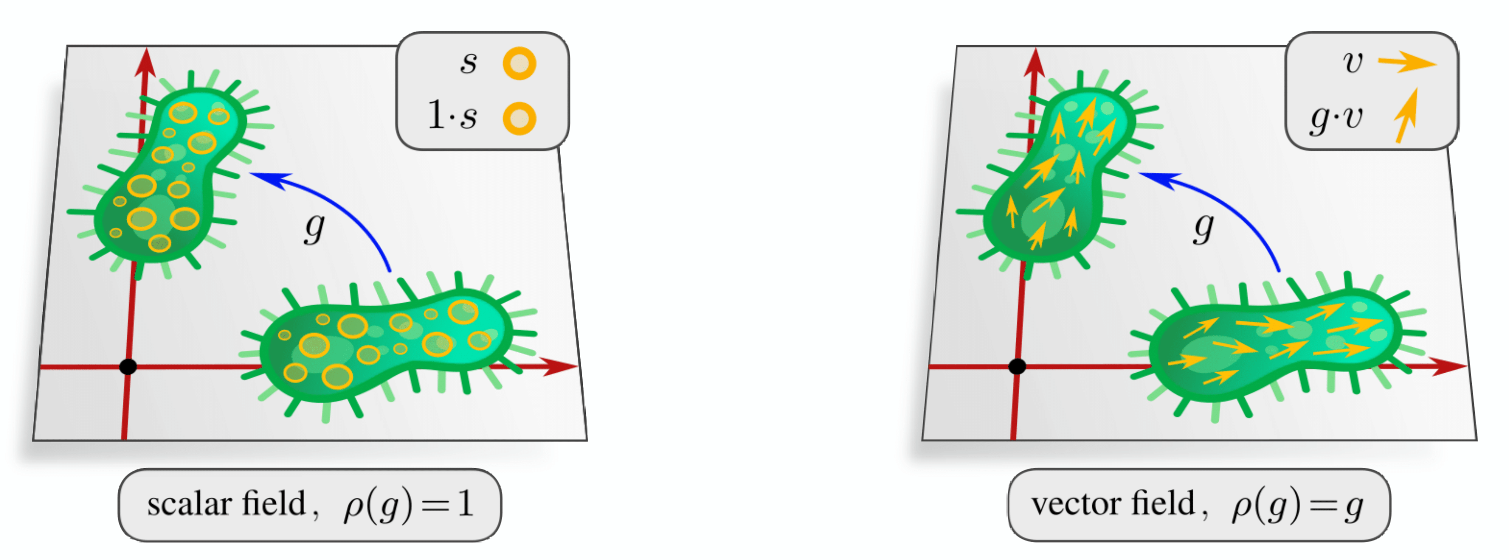
Different types of feature fields: scalar and vector.
Source: escnn.
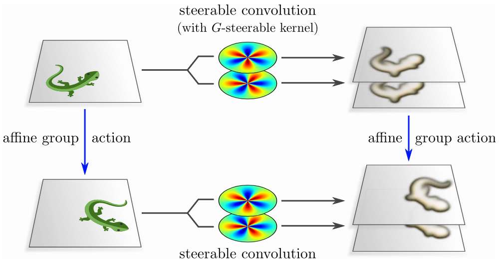
Convolution with \(G\)-steerable kernels commutes with group action.
Source: Maurice's book.
Equivariant (Steerable) CNNs
If we now want to learn a map \(F: f_{\text{in}} \to f_{\text{out}}\), we must respect the geometry of the space. Consequently, the map should respect the transformation laws of the feature fields, which imposes the equivariance constraint: \[ F \circ \rho_\text{in}(g) = \rho_{\text{out}}(g) \circ F. \] This is nothing but a consistency requirement: the function should work the same way regardless of the symmetry transformation applied to the input.
Standard CNNs are already translation equivariant by design, as the same kernel is applied at each location in the input. A lot of work has been done to extend this to the full set of isometries of the Euclidean space, leading to the framework of Steerable CNNs. The core idea here is to use the convolutional operator, as it guarantees translation equivariance, and constrain the space of kernels to be \(O(p,q)\)-equivariant. More formally, a kernel \(k\) should satisfy the following property, called steerability constraint: \[ k(gx) = \rho_{\text{out}}(g) k(x) \rho_{\text{in}}(g)^{-1}. \] The procedure then would be to solve the constraint by hand, obtain the kernel basis, and simply use it in the standard CNN. This approach is general, although quite elaborate, as one needs to solve the constraint for every group of interest \(G\).
Implicit steerable kernels
A viable alternative to solving the steerability constraint by hand is to solve it implicitly. In a nutshell, one only needs to parameterize the kernel as a function using a \(G\)-equivariant MLP, and the resulting convolution is theoretically guaranteed to be \(G\)-equivariant (see the paper for more details). The idea here is to compute the kernel matrix for each point of the kernel grid. In other words, we use the original definition of a kernel as a function: \[ k: \mathbb{R}^{n} \to \mathbb{R}^{c_{\text{out}} \times c_{\text{in}}} \] where \(\mathbb{R}^{n}\) is the n-dimensional base space, and \(c_{\text{out}}, c_{\text{in}}\) are the number of output and input channels. Thus, implicit kernels take a relative position as input and output the corresponding kernel matrix in vectorized form. This operation is efficient as it is done in parallel for all points in the kernel grid and can be cached during inference.
Implicit kernel approach is very general and spares us from solving the steerability constraint by hand. This is especially valuable for pseudo-Euclidean groups, as no general solution exists. Besides, implementing \(G\)-equivariant MLPs is often a lot easier and plenty of ways to do so exist. Ideally, for our specific case of \(O(p,q)\)-equivariant CNNs, we would like to have a way to build an \(O(p,q)\)-equivariant MLP for any \(p,q\) within a single framework. This is the reason why we employ Clifford algebra based neural networks, as they generalize to any \(p,q\).
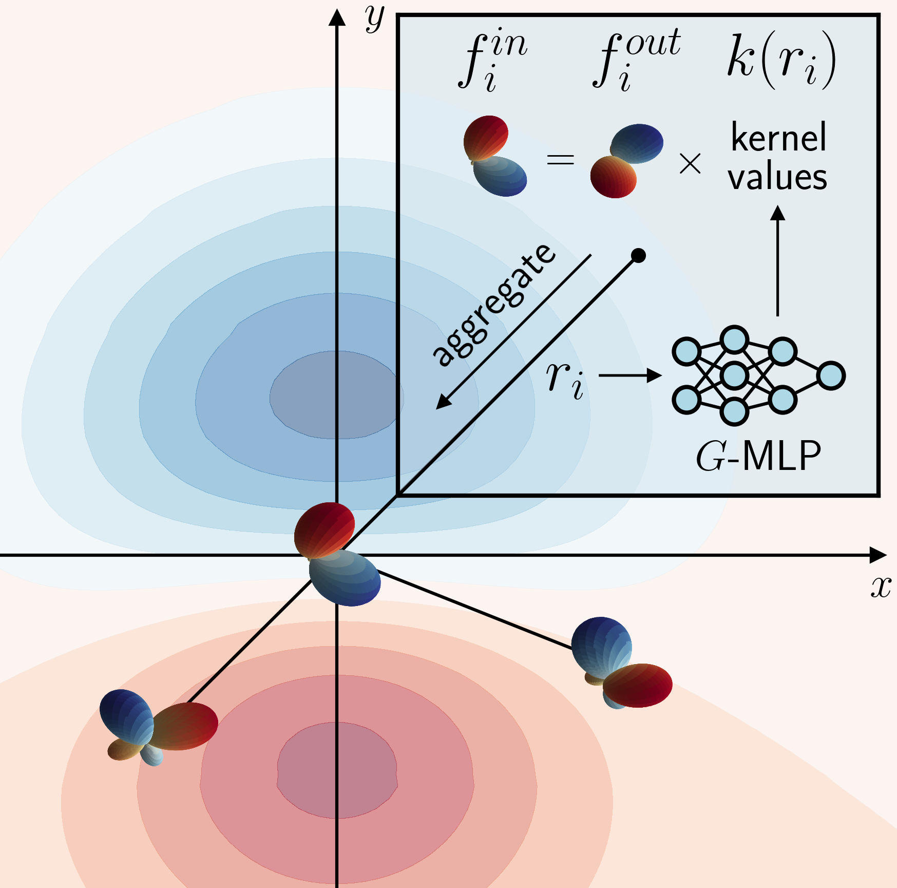
\(G\)-equivariant MLP computes the kernel matrix for each point of the space.
Source: Implicit Steerable kernels paper.
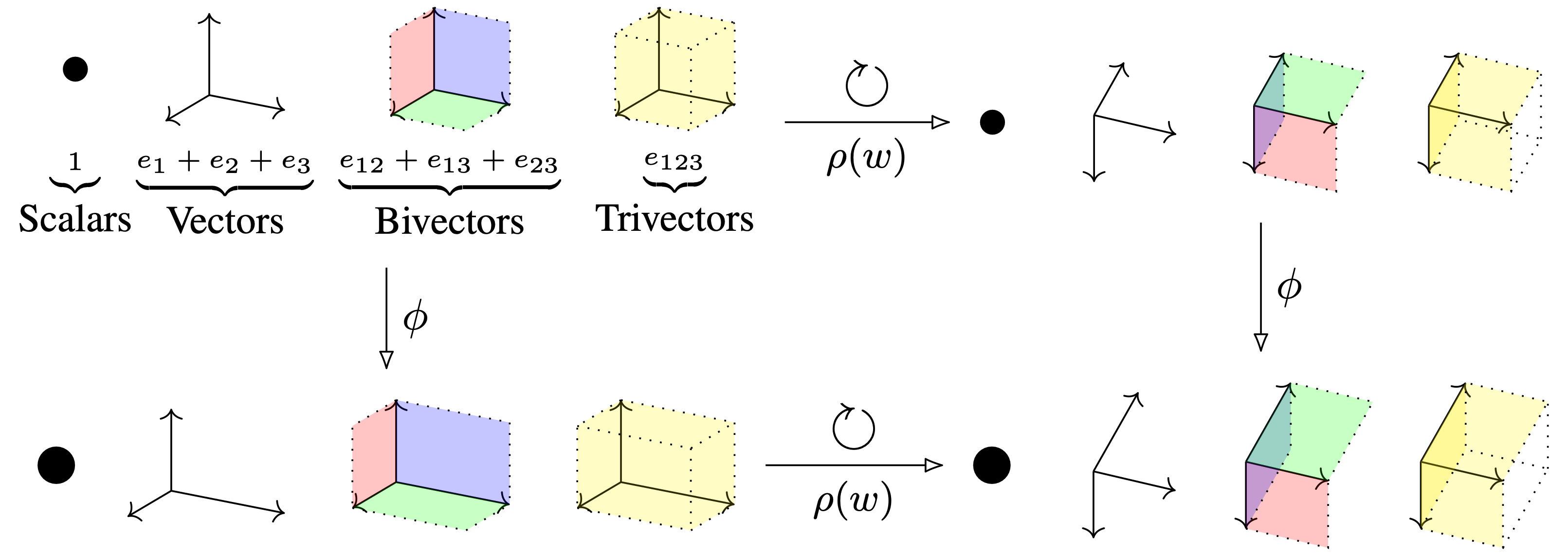
CGENNs operate on multivectors in an \(O(p,q)\)-equivariant way.
Source: Clifford Group Equivariant NNs.
Clifford Group Equivariant NNs
We employ Clifford-algebra based neural networks as they allow very easily to build \(O(p,q)\)-equivariant MLPs (see the CEGNN paper for more details). The main advantage is that the framework trivially generalizes to pseudo-orthogonal groups \(O(p,q)\) regardless of the dimension or metric signature of the space. Furthermore, it is possible to have a single implementation of an \(O(p,q)\)-equivariant MLP, which ultimately allows us to build \(E(p,q)\)-equivariant CNNs within a single framework.
The core idea of CEGNNs is to build the nonlinear map by first applying a linear transformation of each grade of the input multivector, and taking the geometric product with the original input. As geometric product is equivariant, the resulting map is \(O(p,q)\)-equivariant. Nonlinearities are efficiently implemented through a gating mechanism: a standard non-linearity (e.g., ReLU) is applied to the scalar part of the multivector, and the result is then multiplied with the original multivector.
Clifford-Steerable CNNs
Let us do a revision of what we have so far. We learned that we can build \(O(p,q)\)-equivariant CNNs by employing implicit steerable kernels given we know how to parameterize them. A possible choice for the parameterization are \(O(p,q)\)-equivariant MLPs taken from the CEGNN framework. This essentially means that we have to work with multivector fields \[ f: \mathbb{R}^{p,q} \to \text{Cl}(p,q) \] and convolve them with \(O(p,q)\)-equivariant multivector kernels via the geometric product (see the Clifford Neural Layers paper for more details).
The key challenge here is to implement the convolution efficiently, as it does not immediately fit into the standard CNN implementation (due to geometric product instead of matmuls). The issue is solved by partially evaluating the geometric product with the kernel as left input \[ \text{GP}(k, f) \rightarrow K \cdot f \] \[ K = k \cdot \text{Cayley table} \] where Cayley table essentially says how grades of two input multivectors interact with one another and produce the output multivector. This transformation casts the bilinear operation (geometric product) into a linear one (matmul), which is exactly what traditional CNNs use. Now let's look at the implementation in detail.
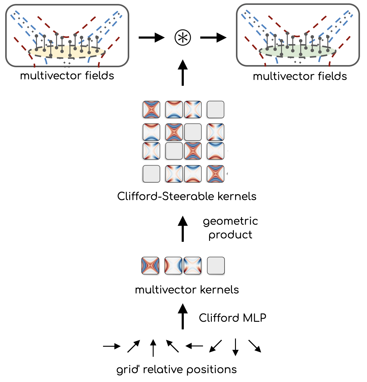
Multivector kernels are computed at each point of the grid, and then the geometric product is partially evaluated to yield Clifford-Steerable kernels.
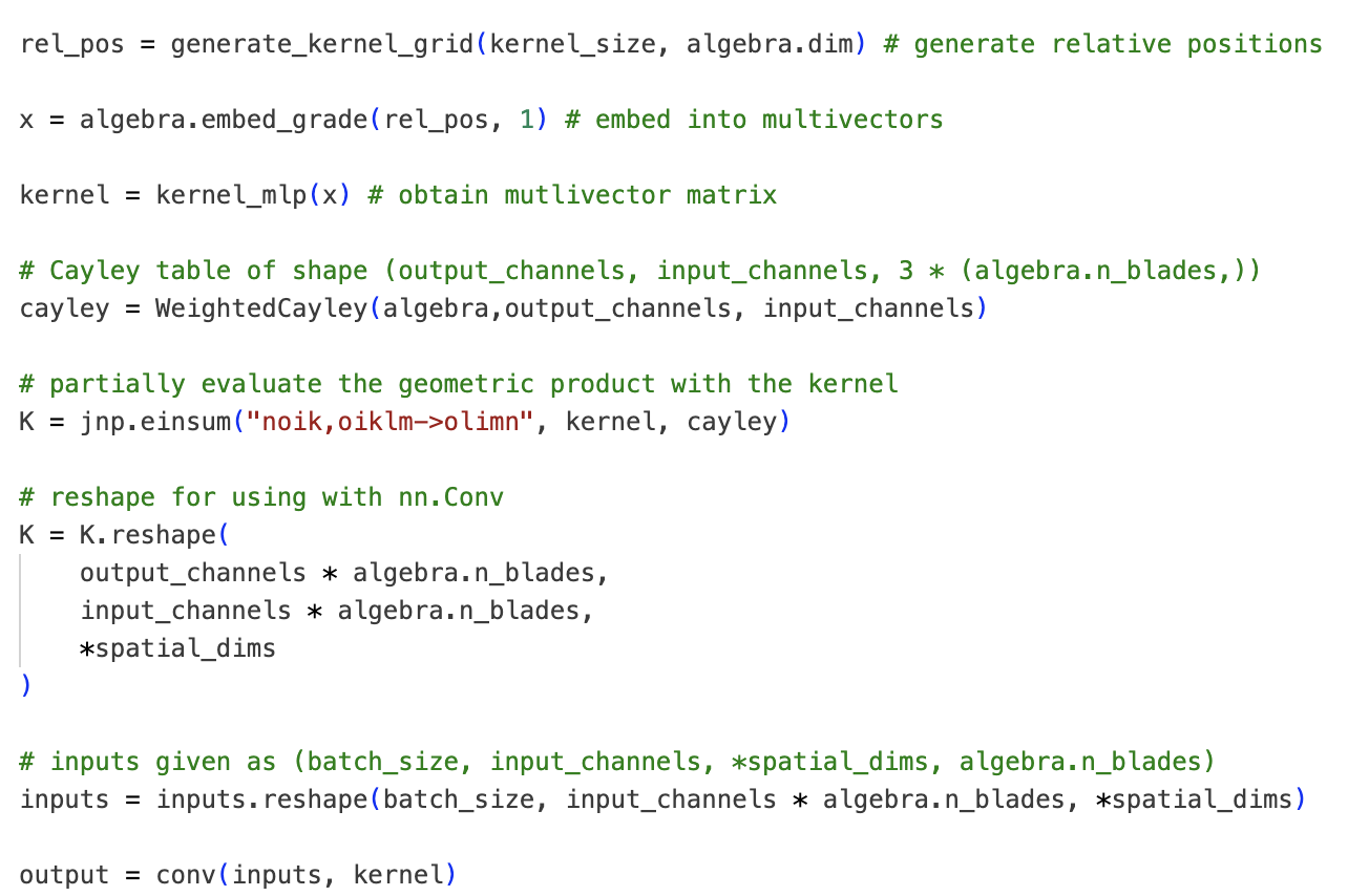
Simplified pseudocode.
Implementation
The way the implicit kernels works is given below:
- Given kernel size, discretize \([-1,1]^{p+q}\) to compute the grid as relative positions.
- Embed the relative positions as vector part of multivectors \(\to\) batch.
- Compute multivector matrices (vectorized) for each element of the batch.
- Partially evaluate the geometric product by multiplying the batch of matrices with Cayley table of the algebra.
- Reshape the output to \((C_{\text{out}} \cdot 2^{p+q},C_{\text{in}} \cdot 2^{p+q}, X_1, ..., X_{p+q})\).
- Given: input multivector field of shape \((B, C_{\text{in}}, X_1, ..., X_{p+q}, 2^{p+q})\).
- Compute the kernel as described above.
- Reshape the input field to \((B, C_{\text{in}} \cdot 2^{p+q}, X_1, ..., X_{p+q})\).
- Perform the convolution operation \(\to\) output multivector field of shape \((B, C_{\text{out}} \cdot 2^{p+q}, X_1, ..., X_{p+q})\).
- Reshape the output field to \((B, C_{\text{out}}, X_1, ..., X_{p+q}, 2^{p+q})\).
Experiments
We evaluated our model on three forecasting tasks: Navier-Stokes on \(\mathbb{R}^{2}\), Maxwell's equations on \(\mathbb{R}^{3}\), and relativistic electrodynamics on \(\mathbb{R}^{1,2}\) (dataset available here). The primary difference between these tasks is that in the first two, time steps are treated as feature channels, while in the last one, time is a separate dimension, i.e. part of the grid. For the first two tasks, a single time step is predicted from 4 previous ones, while for the last one, 16 previous time steps are mapped to 16 future ones. All models have similar number of parameters.
First thing to notice is the extreme sample complexity of CS-CNNs. Compared to standard CNNs, they need 80x less training simulations to reach the same performance on the Navier-Stokes task. Besides, for the given parameter count, we did not observe non-equivariant models to catch up with CS-CNNs as the number of training simulations increases.
Second, CS-CNNs generalize to arbitrary isometries of the base space, hence they work out of the box for any orientation of the grid. Moreover, in the relativistic case, the boost-equivariance of CS-CNNs results in more stable feature fields when viewed from the comoving frame.
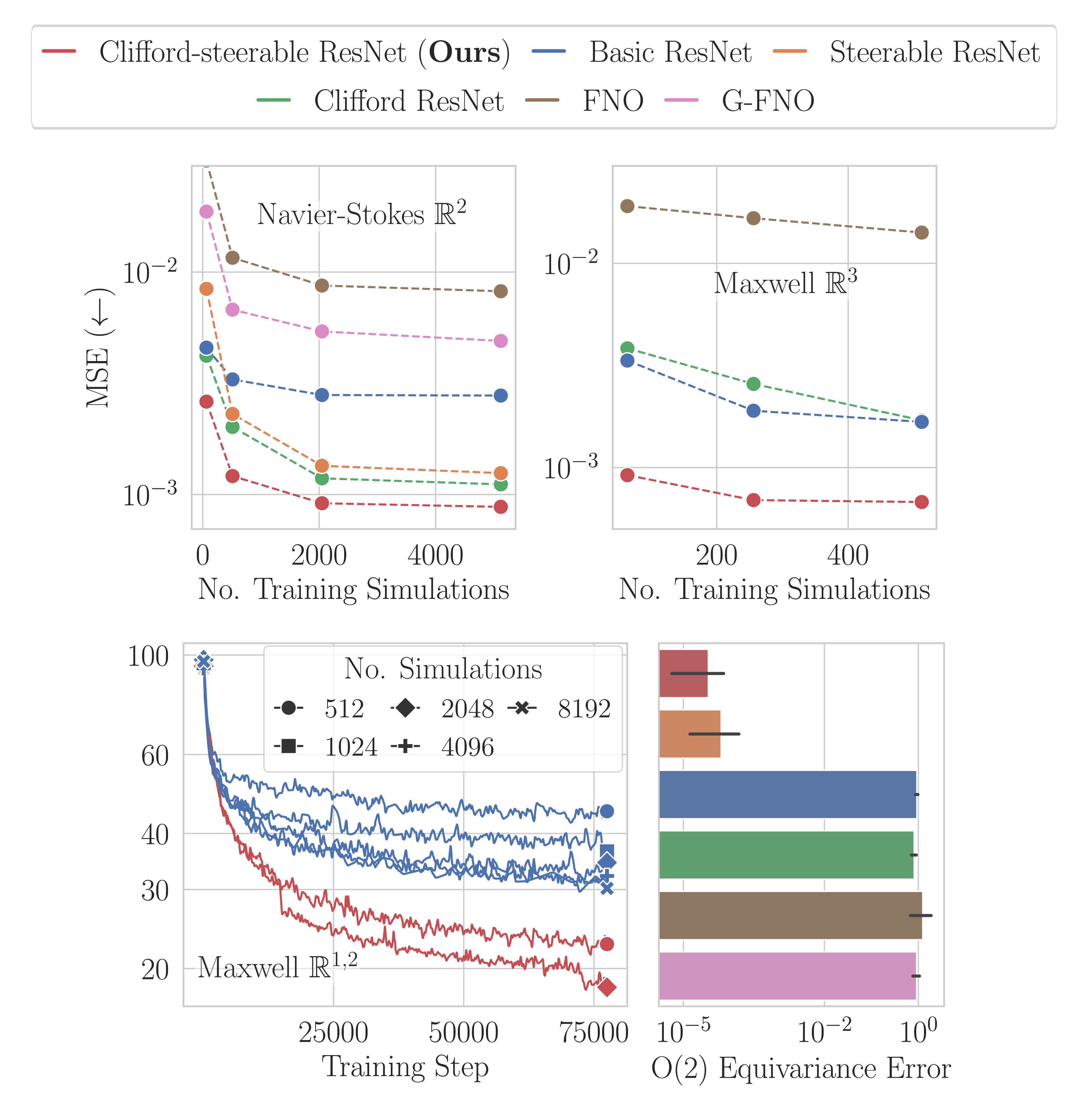
MSE on different forecasting tasks (one-step loss) as a function of number of training simulations.
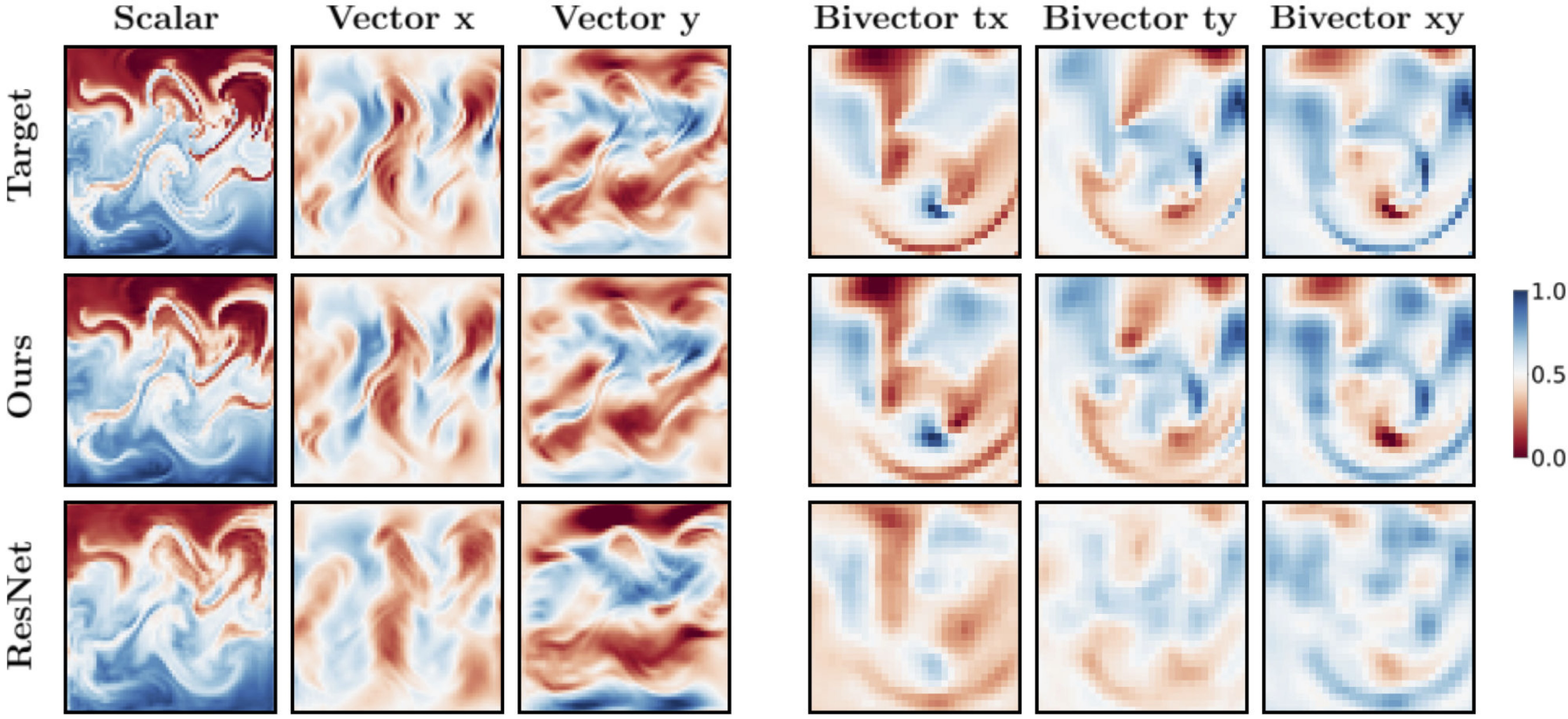
Visual comparison of
target and predicted fields.
Left: Navier-Stokes. Right: Relativistic electrodynamics.
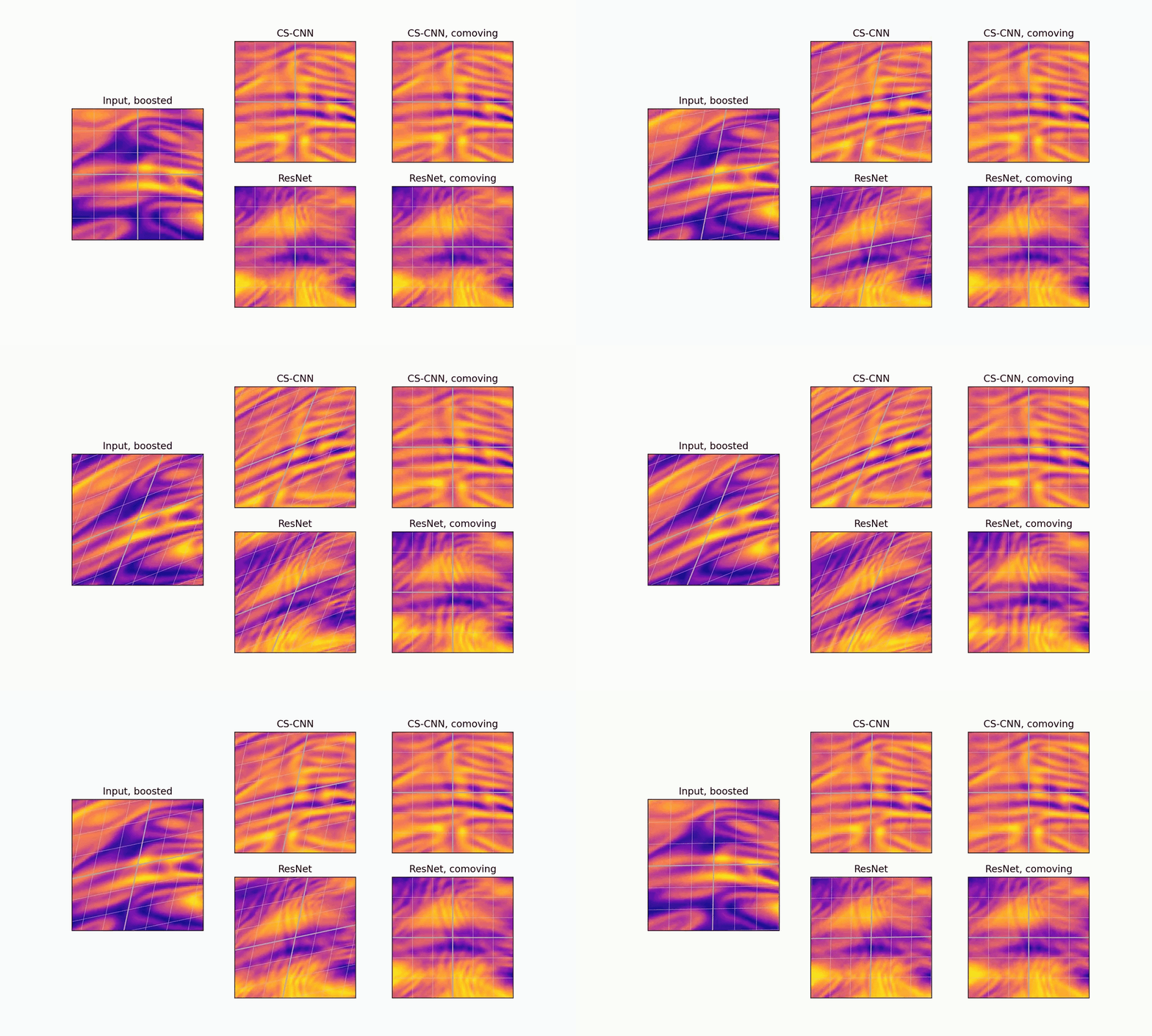
Boost-equivariance: our model produces consistent predictions that are stable when viewed from the comoving frame. ResNet is not boost-equivariant and produces inconsistent predictions.
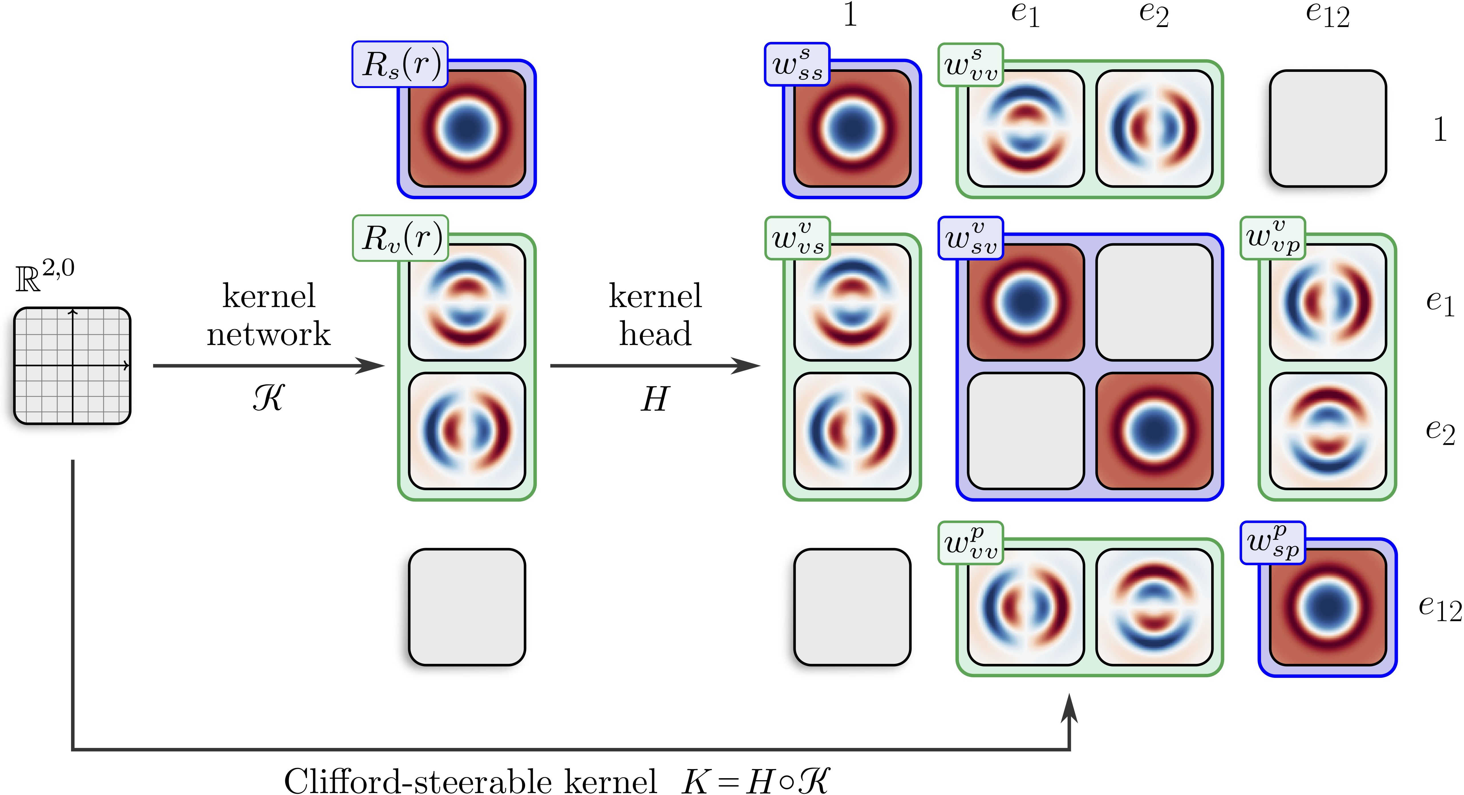
Compared to the Steerable CNNs, the kernel basis of CS-CNNs misses certain degrees of freedom.
Miscellaneous
- Multivector representations: multivectors are not able to represent irreps with frequencies higher than 1. This can be illustrated using the (O(3)) group: the vector/bivector part of a multivector is 3-dimensional, whereas irreps with angular frequency 2 are 5-dimensional. It follows that it is not possible neither to represent such irreps (e.g. a tensor) nor to learn a map that involves them. The latter is precisely the reason why the kernel basis of CS-CNNs is not complete - vector to vector mapping requires frequency 2 kernels, which are not present in the basis. This issue is, however, alleviated when applying multiple convolutional layers, which recover the missing degrees of freedom (see Appendix B in the paper for proof).
- Kernel's input: the kernel's input is limited to the relative position and its norm (shell), which form the 0- and 1-grade components of the input multivector. With this input, the CEGNN backbone is theoretically not able to learn multivectors with non-zero 2-grade. Precisely, the reason for that is that 2-grade appears from the interaction of two unique 1-grades, which is not possible as only one 1-grade is present in the input. There are, of course, ways to overcome this limitation, which we did not explore in this work, but I would be happy to chat about it.
Overall, a lot of work can be done to improve the model, both at the high level (improving expressivity of implicit kernels) and at the low level (developing more expressive basis based on multivectors). Let me know if you are interested in collaboration or just want to chat about the paper :)
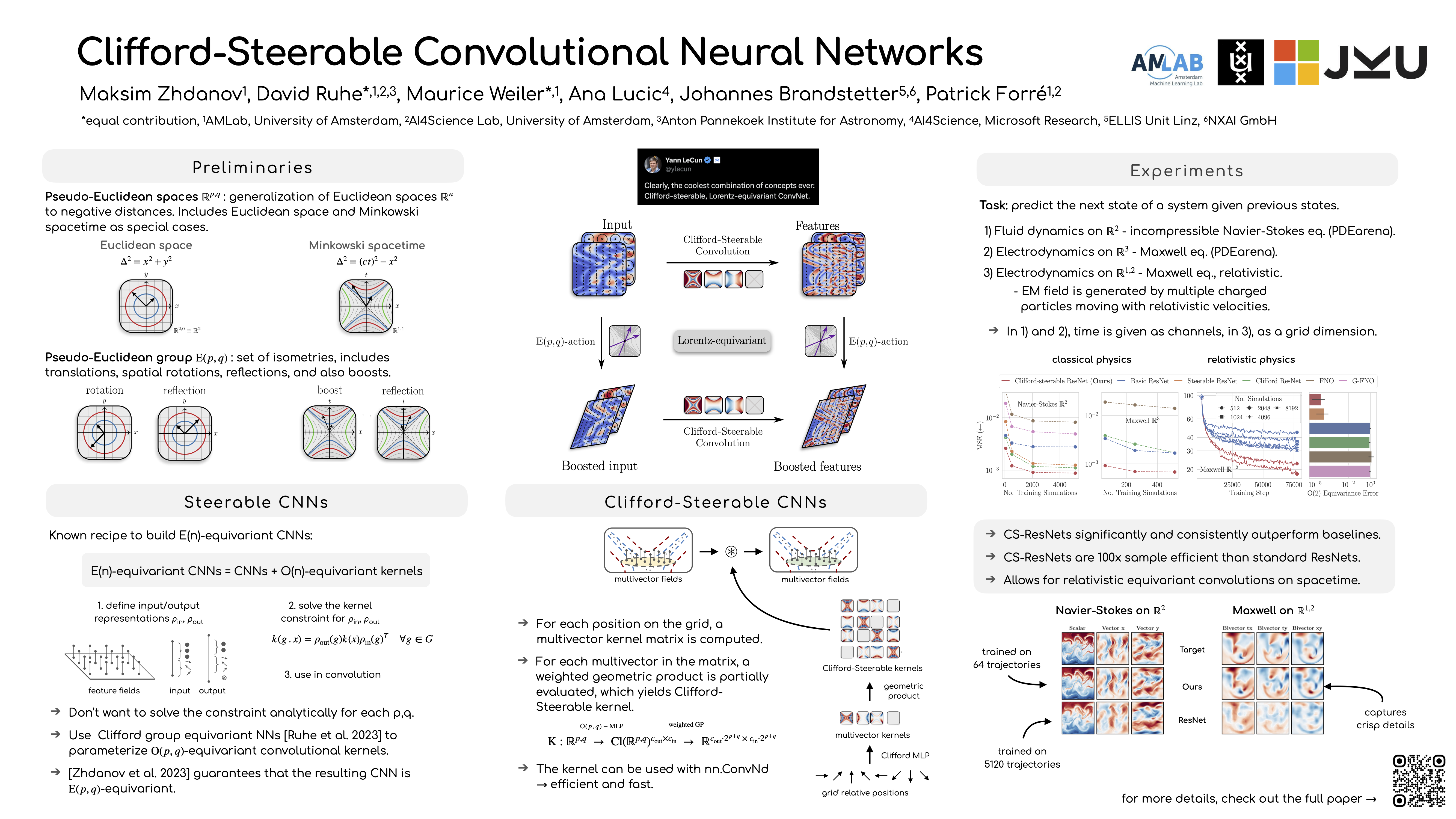
Poster
BibTeX
      @inproceedings{
        Zhdanov2024CliffordSteerableCN,
        title = {Clifford-Steerable Convolutional Neural Networks},
        author = {Maksim Zhdanov and David Ruhe and Maurice Weiler and Ana Lucic and Johannes Brandstetter and Patrick Forr{\'e}},
        booktitle = {International {Conference} on {Machine} {Learning} ({ICML})},
        year = {2024},
    }